Camera Calibration

For this activity we would transform the camera coordinates into world coordinates. We used a checkerboard as the calibration object.
Since the board is placed in a 90 degree angle, I assigned the left face as the x-axis, the right face as the y-axis and the vertical axis as the z-axis. Doing this would simplify most of the equations. The origin is place bottom center of the board.
25 cornerpoints were randomly assigned. So that I would not get lost in using the locate function in Scilab, I placed markers in the image. (This would have no effect since we don't need the color information of the image) (NOTE: see code for the coordinates of the points). Each square in the board measures 1x1 inch.
In lecture 2, the camera axis is labeled as x and the image plane as yz. Since the xyz axis can be permutated without affecting the location of a point in the plane, the same derivation can be used but this time change all x with z, all y with x, and all z with y.
To solve for the camera parameters, we used the following equation:
Labeling the first matrix as Q, the second as a (camera parameters), and the third as d (image plane coordinates), we get:
//Scilab code
image = imread("cboard-marked-gs.bmp") - 1;
imshow(image, [])
d = locate(25, flag = 1);
coords = [0 0 0 0 0 0 0 0 0 0 0 0 1 1 1 1 2 3 3 4 5 5 6 6 6; //x
1 1 2 2 3 4 4 4 4 5 6 6 0 0 0 0 0 0 0 0 0 0 0 0 0; //y
2 6 4 7 5 1 3 6 9 7 3 5 1 3 5 8 6 2 8 4 2 7 1 4 9]; //z
Q = [];
for i = 1:25
x = coords(1, i);
y = coords(2, i);
z = coords(3, i);
yi = d(1, i);
zi = d(2, i);
Qi = [x y z 1 0 0 0 0 -(yi*x) -(yi*y) -(yi*z);
0 0 0 0 x y z 1 -(zi*x) -(zi*y) -(zi*z)];
Q = cat(1, Q, Qi);
end
d = matrix(d, [length(d), 1]);
a = inv(Q'*Q)*Q'*d
//end of code

The computed camera parameters are:
-19.387751
9.411270
-0.564041
172.318473
-2.744767
-3.956096
20.590540
36.630648
-0.008846
-0.013345
-0.001769

To this if this calibration is correct, I first tried to convert the object coordinate to image coordinate using the camera calibration above and the following equation:
//Scilab code
a = [-19.387751 ;9.411270 ;-0.564041 ;172.318473 ;-2.744767 ;-3.956096 ;
20.590540 ;36.630648 ;-0.008846 ;-0.013345 ;-0.001769 ]
coords = [0 0 0 0 0 0 0 0 0 0 0 0 1 1 1 1 2 3 3 4 5 5 6 6 6;
1 1 2 2 3 4 4 4 4 5 6 6 0 0 0 0 0 0 0 0 0 0 0 0 0;
2 6 4 7 5 1 3 6 9 7 3 5 1 3 5 8 6 2 8 4 2 7 1 4 9];
yi = []
zi = []
for i = 1:6
x = coords(1, i);
y = coords(2, i);
z = coords(3, i);
yi(i) = (a(1)*x + a(2)*y + a(3)*z + a(4))/(a(9)*x + a(10)*y + a(11)*z + 1);
zi(i) = (a(5)*x + a(6)*y + a(7)*z + a(8))/(a(9)*x + a(10)*y + a(11)*z + 1);
end
d = cat(2, yi, zi);
//end of code

After processing all the coordinates used, the deviations from using the locate function of scilab and this equation are:

yi	zi
0.52826	0.87672
0.87410	0.22682
0.15622	0.77860
0.83752	0.86413
0.84163	0.82441
0.64452	0.62763
0.89180	1.10098
0.33847	0.09812
0.41275	0.15379
0.37815	0.40735
0.66961	0.21872
0.87220	0.29042
0.83183	0.46501
0.87415	1.30520
0.98954	0.23742
0.01032	0.98742
1.06601	0.00136
0.50450	0.61056
0.42662	0.28194
0.77159	0.11263
0.87657	0.02865
0.11396	1.14443
1.33988	0.06806
0.99433	1.24125
0.22386	0.0234

The mean is 0.659 and 0.519 for yi and zi respectively with standard deviation equal to 0.335 and 0.425. This translates to less than 2% error for all the values computed.
Using the camera parameters obtained, I tried predicting the image coordinates of some unused cornerpoints. The results are as follows:

Predicted			Located			Difference
171.537	98.9273		172.187	98.9699		0.650	0.043
183.460	96.2413		186.133	95.1664		2.674	1.075
208.713	47.3315		209.588	47.6228		0.875	0.291
153.706	76.0082		155.705	76.4342		1.999	0.426
135.287	73.8909		135.42	75.5151		0.133	1.624
115.791	114.611		115.135	113.550		0.657	1.061

The predictions were quite accurate.

For this activity, I give myself a grade of 10 because the results I obtained were precise and accurate.
Thanks to Cole Fabros for some clarifications on the needed equations
Collaborators: Raf Jaculbia

Preprocessing Handwritten Text

For this activity, we would try to extract handwriiten text from scanned tables. From the whole scanned document I cropped the portion shown below:
As can be seen, the text is barely discernible from the image but I'll try my best to extract it :D.
The first thing I did was to get the Fourier transform of the image so that I can make an appropriate filter. Since I wanted to remove the table, I created a filter which would block all the horizontal and vertical lines (shown below).
The image after filtering:
As can be seen, some of the lines still remain but are now white so if I am to binarize the image, most of this would not affect the image.
Since have no program that can estimate the best threshold, I estimated it using trial and error. After thresholding:

Most of the table lines are now gone but some lines still remain in the left side of the image :( And also, most of the text are now unreadable (they were quite unreadable to begin with) and the text in the fourth column are now gone since they were written lightly.
To further enhance the image, I used the opening and closing operators with a 2x2 structuring element. Also to make the width of the letters 1 pixel, I eroded the image with a 2x1 structuring element.
The last thing to do was to label the letters.
The total labeled blobs was 256 which was very high compared to the number of letters appearing in the text. This was expected since as we can see in the image, there are lots of pixels which do not correspond to any text or a single letter is broken up to many pieces.

//Scilab code
image1 = imread("text-fft-filter3.bmp") - 1;
image2 = imread("text.bmp") - 1;
se1 = imread("se1.bmp"); //a 2x1 structuring element
se2 = imread("se3.bmp"); // a 2x2 structuring element

fftimage1 = fftshift(image1);
fftimage2 = fft2(image2);

image1_2 = fftimage1.*fftimage2;
infft = fft2(image1_2);
fimage = real(infft);
fimage = (fimage/max(fimage)) * 255;
[x, y] = histogram(fimage);
scf(1);
imshow(fimage, []);
//bar(x,y)
threshold = (find(y == max(y), 1) - 30)/255;
image = im2bw(fimage, threshold);
scf(2);
imshow(image, [])
image = abs(image - 1);

//Opening
image = dilate(erode(image, se2, [1,1]), se2, [1,1]);

//Closing
image = erode(dilate(image, se2, [1,1]), se2, [1,1]);

image = erode(image, se1, [1,1]);

scf(3);
imshow(image, []);

labeled = bwlabel(image, 4);
scf(4);
imshow(labeled, []);
//end of code

For this activity, I give myself a grade of 9 since I can't find the proper threshold for the image.
Collaborators: None

Binary Operations

For this activity, we need to measure the area (in pixel counts) of a punched paper. The image I used is shown below. I then subdivided the entire image into 10 256x256 sub-images so that scilab can process the images better. Because the morphological operations that we know only works for binary images and the image given was still in grayscale, I converted it using a threshold. The threshold I used was near the max of the histogram of the grayscale image.
To better represent the circles, I used the closing operator (done by eroding the dilation of the image) first then the opening operator (dilating the erosion of the images). The structuring element used was a 2 pixel radius circle. After cleaning the image with opening and closing operator, I used the bwlabel of scilab to tag the blobs found in the image. The area of each blob is then measured by pixel counting.
//Scilab code getf("imagehist.sce");
image = imread("C1_10.bmp") - 1;
se1 = imread("se2.bmp");
[x, y] = histogram(image);
threshold = (find(y == max(y), 1) - 1 + 30)/255;
image = im2bw(image, threshold);

//Opening
image = dilate(erode(image, se1, [1,1]), se1, [1,1]);
//Closing
image = erode(dilate(image, se1, [1,1]), se1, [1,1]);

labeled = bwlabel(image, 4);
imshow(labeled, []) iteration = max(labeled);
sizes = []; for i = 1:iteration blob = find(labeled == i);
sblob = size(blob);
sizes(i) = sblob(2);
end
//end of code

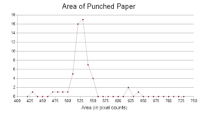
After pixel counting, I obtained the following histogram:
The points below 400 and above 700 were not shown since they have only a frequency of 2 or less. Also, by not showing these points, the graph has been "zoomed" to values with high frequencies.
The histogram shows that the area of single punched paper is near 520-530 pixels. To verify if this value is correct, I measured the diameter of a single punched paper using GIMP. The diameter measured is approximately 26pixels. So inserting this value to the area equation for circle (pi * r^2), the area is 531 pixels which is very near to the peak of the histogram. Another method used was to pixel count an image of single punched paper. Using this method, the area was calculated to be equal to 538 pixels which is still near the peak. The mean and standard deviation of the areas calculated near the peaks (300 - 700 pixels) were also calculated. Only these values were considered because I think that computed areas lower than 300 are the circles which were truncated and those greater than 700 are 2 or more overlapping circles counted as a single blob. The computed mean was equal to 510 pixels with standard deviation equal to 56 pixels. The peak in the histogram is still within this range.

For this activity, I give myself a grade of 10 because I was able to do it properly.
Collaborator: Raf Jaculbia

Morphological Operations

For this activity, we analyzed the morphological operations done on binary images, specifically dilation and erosion. The first thing that we did was to predict using hand-drawn images the effects of different structuring elements on the binary images. The structuring elements used and the diolation/erosion predictions can be seen in the drawings below.
To verify if these predictions were correct, these morphological operations were also done in scilab.
//Scilab code
image = imread("50x50square.bmp");
se1 = imread("se1.bmp");
se2 = imread("se2.bmp");
se3 = imread("se3.bmp");
se4 = imread("se4.bmp");

d1 = dilate(image, se1, [1,1]);
d2 = dilate(image, se2, [1,1]);
d3 = dilate(image, se3, [1,1]);
d4 = dilate(image, se4, [3,3]);

//For erosion, just uncomment the following lines
//d1 = erode(image, se1, [1,1]);
//d2 = erode(image, se2, [1,1]);
//d3 = erode(image, se3, [1,1]);
//d4 = erode(image, se4, [3,3]);

subplot(332);
imshow(image, []);

subplot(334);
imshow(d1, []);

subplot(336);
imshow(d2, []);

subplot(337);
imshow(d3, []);

subplot(339);
imshow(d4, []);
//end of code

For the following images, the uppermost image is the original image. The upper left image is the image operated using B1(see drawing), upper right is operated using B2, lower left is operated using B3, and lower is operated using B4.
Square
Dilation

Erosion

Triangle
Dilation
Erosion
Circle
Dilation
Erosion
Hollow Square
Dilation
Erosion
Cross
Dilation
Erosion
Looking at the images produced by scilab, it looks like my predictions were correct.

For this activity, I give myself a grade of 10 because I did the predictions first before making the scilab code and my predictions were quite accurate. Also, I would like to thank Elizabeth Prieto for clarifying some concepts.

Enhancement in the Frequency Domain

The first part of this activity involves studying the some more properties of the Fourier transform. The images below shows a 2D sinusoidal function and its Fourier transform . As can be seen in the images, the maximum in the frequency domain is perpendicular to the direction of the sinusoid. So, as the sinusoid is rotated, the Fourier transform also rotates.

The second parameter investigated was the frequency of the sinusoid used. From the images below we can see that as the frequency is increased, the separation between the points (which corresponds to the black and white stripes) become larger.
Ridge Enhancement
In this activity, we would try to enhance the ridges in a fingerprint by filtering the frequency domain. I used the fingerprint found in the pdf since the fingerprint I scanned was small and so the results are not noticeable. The Fourier transform of the fingerprint and the filter mask I used is shown below. The filter was designed such that the low frequencies in the image are blocked.
After filtering (images below), the ridges in the fingerprint images were enhanced (upper right) but blotches are still present. However, if we take only the real part of the inverse Fourier transform of the filtered Fourier transform, the blotches are almost gone while still maintaining the same ridge quality.


Line Removal
For this activity, we were given an image of the moon with lots of vertical lines in it. Our task is to remove it using filters in the frequency domain. From our past activity, I learned that vertical lines are seen as horizontal lines in the frequency domain. So, I designed a frequency filter which would block these horizontal lines. The fourier transform of the image is shown in the upper left figure and the filter used is shown in the upper right. The original and line removed images are shown below. (left and right respectively)

I give myself a grade of 8 for this activity since I'm not sure if I did the ridge enhancement properly.

Fourier Transform Model of Image Formation

For this activity, we analyzed the different properties and uses of the Fourier transform. Our first task was to get the Fourier transform of a circle and the letter A.
As we can see in the figures, as the circle becomes small, more airy disc appear in the Fourier space. Also, this result is similar to the analytic Fourier transform of a circle which is an equation of the airy disc.
The next image used was a letter A as shown above (left figure). The Fourier transform (center) has an X and a vertical line. The X line corresponds to the orientation of the legs of A while the vertical line corresponds to the general orientation of the letter (i.e. if the letter is rotated 90 degrees, the Fourier transform would have a horizontal line instead of vertical). The last image (right) is the fft of the fft of the image. It is inverted because a forward fft was used instead of the inverse fft.

The next activity was to get the convolution of an image with a circle. We used the word VIP as the image and I used the circles I used above.

Since convolution is like mixing the images together, we can see that the larger the aperture (circle) the clearer the object. This happens because the Fourier transform of a small aperture produces more airy disc therefore contributing more to the final image.

To find identical patterns, we used correlation. This was done by multiplying element wise the conjugate of the Fourier transform of the text image (left) with the Fourier transform of the pattern that we wanted to find, in this case the letter A (middle figure). The resulting image (right) have a maximum (white) where the letter A appears in the text.

The concept used in correlation was modified to find edges in images. I used a horizontal, vertical, and spot pattern.
The detected edges mostly follows the pattern used. For the horizontal pattern (left) the convolve image has mostly horizontal edges, the vertical has mostly vertical edges, and the spot pattern detects both horizontal and vertical edges.

For this activity, I give myself a grade of 10 because I did the activity properly and independently.

Physical Measurements from Discrete Fourier Transforms

In this activity, we examined the Fourier transforms of signals. The first signal used was a 1-D sinusoidal function. The sine function and its Fourier transform is shown below.

To get a Fourier transform of an image, we just need to use the 2-D form of the DFT. Since the magnitude of the Fourier transform contains most of the geometric information of the spatial domain image, it was displayed as the final image.

To accurately measure the FT of a fluorescent bulb, which flickers at around 120Hz, we need at least dt = 1/240 sec. This was obtained using the Nyquist formula, fmax = 1/(2*dt), where fmax is the maximum frequency the FT can detect without aliasing. So setting fmax = 120Hz, we get dt = 1/240 sec.

Effects of N and dt in the frequency domain.
The discrete frequency steps (df) in the frequency domain is given by df = (2*fmax)/N. So if N is increased, the frequency domain would be much more sensitive to small frequencies and it would be more accurate since there is a smaller frequency samples.
From the plots obtained(left: N = 256, right N = 1024), it can be seen that higher N results in a more accurate(narrower) value in the frequency domain. Although both peaks at 5, which is the frequency of the signal used, with N = 256, the plot range is 4.5-5.5 while with N = 1024, it is 4.9-5.1.
Combining the Nyquist theorem with the discrete frequency equation, we get df = 1/(dt*N). So as dt approaches 0, df approaches infinity. Therefore, I expect that decreasing dt would result in a less accurate(broader) frequency plot.
The plots obtained(left: dt = 2/256, right: dt = 2/64) shows that the expected results were correct.

For this activity, I give myself a grade of 10 since I performed all of the required activities.