For this activity, we did another image classification based on neural networks. A neural network consists of 3 parts, an input layer, where in our case contains the features of an object class, a hidden layer, where the features are compared, and an output layer, which gives what class the object belongs. The output of the neural network I made is either 0(class 1) or 1(class 2) depending on what class the object belongs.
For comparison with other techniques, I used the same data as the previous activities(probabilistic classification and pattern recognition).
For this method, I also obtained a 100% correct classification.
Program Output:
0.0000048 0.0000250 0.0002727 0.0351369
0.9999835 0.999997 0.9999921 0.9684366
Rounding this numbers off gives 0 for the first 4 test and 1 for the next 4 which is correct since the first 4 images were taken from class 1 and the others from class 2.
//Scilab code
//4 neurons in the input layer, 32 in the hidden layer and 1 in the ouput layer
N = [4,32,1];
// Training Set
x = [3730,0.526882,0.475084,0.394192;
4277,0.630000,0.455594,0.388616;
4181,0.656250,0.462898,0.386272;
4262,0.744186,0.479152,0.397529;
3876,0.868421,0.564352,0.331341;
3576,0.888889,0.522656,0.339387;
3754,0.893333,0.525226,0.349733;
4161,0.802469,0.503910,0.352362]';
normalizer = max(x(1,:)); //to reduce the magnitude of the area
x(1, :) = x(1, :)./normalizer;
t = [0 0 0 0 1 1 1 1];
lp = [2.5,0];
W = ann_FF_init(N);
//Training cyles
T = 1000;
W = ann_FF_Std_online(x,t,N,W,lp,T);
//x is the training t is the output W is the initialized weights,
//N is the NN architecture, lp is the learning rate and T is the number of iterations
test = [3730,0.526882,0.475084,0.394192;
4277,0.630000,0.455594,0.388616;
4181,0.656250,0.462898,0.386272;
4262,0.744186,0.479152,0.397529;
3876,0.868421,0.564352,0.331341;
3576,0.888889,0.522656,0.339387;
3754,0.893333,0.525226,0.349733;
4161,0.802469,0.503910,0.352362]';
test(1, :) = test(1, :)./normalizer;
ann_FF_run(test,N,W)
//Code end
I give myself a grade of 10 since I was able to correctly use and modify the given program.
Tuesday, September 30, 2008
Thursday, September 18, 2008
Probabilistic Classification
In this activity, we did another method in image classification, Linear Discrimination Analysis. (In-depth tutorial can be found at http://people.revoledu.com/kardi/tutorial/LDA/LDA.html) The main idea of this point is to find an axis rotation where the features of a class can be grouped together while making it far away as possible from the features of the other classes,very much similar to what is done in principal component analysis(PCA). The inputs are object samples(rows in variable x), object features(columns in x) and object class(variable y). I used 2 classes from the pattern recognition activity, squidballs and piatos (since the misclassification in that activity happened between these classes). The features are area, height/width, average red (NCC) and average green (NCC). The training set is as follows:
Class 1 is piatos and class 2 is squidball. After some calculations, I obtained the covariance matrix which is equal to:
| Area | height/width | Red | Green | Class |
| 3730 | 0.526882 | 0.475084 | 0.394192 | 1 |
| 4277 | 0.630000 | 0.455594 | 0.388616 | 1 |
| 4181 | 0.656250 | 0.462898 | 0.386272 | 1 |
| 4262 | 0.744186 | 0.479152 | 0.397529 | 1 |
| 3876 | 0.868421 | 0.564352 | 0.331341 | 2 |
| 3576 | 0.888889 | 0.522656 | 0.339387 | 2 |
| 3754 | 0.893333 | 0.525226 | 0.349733 | 2 |
| 4161 | 0.802469 | 0.503910 | 0.352362 | 2 |
| 66054.609375 | -11.454640 | -5.145901 | 3.528965 |
| -11.454640 | 0.016200 | 0.003636 | -0.002744 |
| -5.145901 | 0.003636 | 0.001212 | -0.000800 |
| 3.528965 | -0.002744 | -0.000800 | 0.000632 |
The discriminant can be computed using
 where fi is the linear discriminant, (mu) is the mean feature of class i, C is the covariance matrix, xk is the object feature set to be classified, and p is the probability of class i occuring, which is just the # of objects in class i divided by the total # of objects.
I used the same test images from the activity pattern recognition (first 4 objects were piatos, class 1, and the next 4 are squidballs, class 2). The feature set of the test images is shown below.
Using these test image features, I obtained the following discriminant values:
A positive (f1 - f2) means that an object is classified as class 1 while a negative (f1 - f2) is an object classified as class 2. From the table above the first 4 objects were classified as belonging to class 1 and the next 4 objects were class 2. The results were 100% correct. ^_^ I also tried shuffling the positions of the test objects, because the result might just have copied the arrangement of classes in variable y, and I still get a 100% correct classification.
//Scilab code
x = [3730 0.526882 0.475084 0.394192;
4277 0.630000 0.455594 0.388616;
4181 0.656250 0.462898 0.386272;
4262 0.744186 0.479152 0.397529;
3876 0.868421 0.564352 0.331341;
3576 0.888889 0.522656 0.339387;
3754 0.893333 0.525226 0.349733;
4161 0.802469 0.503910 0.352362];
xt = [4717 0.888889 0.472711 0.398525;
4870 0.663265 0.470151 0.375207;
5709 0.647619 0.462389 0.382276;
5554 0.666667 0.474319 0.375255;
4144 0.960526 0.519057 0.361193;
3503 0.912500 0.461393 0.370681;
3985 1.000000 0.499096 0.365295;
4592 1.111111 0.473050 0.352714];//classes to test, 1-4 class 1, 5-8 class 2
y = [1;
1;
1;
1;
2;
2;
2;
2];
x1 = [3730 0.526882 0.475084 0.394192;
4277 0.630000 0.455594 0.388616;
4181 0.656250 0.462898 0.386272;
4262 0.744186 0.479152 0.397529];
x2 = [3876 0.868421 0.564352 0.331341;
3576 0.888889 0.522656 0.339387;
3754 0.893333 0.525226 0.349733;
4161 0.802469 0.503910 0.352362];
n1 = size(x1, 1);
n2 = size(x2, 1);
m1 = mean(x1, 'r');
m2 = mean(x2, 'r');
m = mean(x, 'r');
x1o = x1 - mtlb_repmat(m, [n1, 1]);
x2o = x2 - mtlb_repmat(m, [n2, 1]);
c1 = (x1o'*x1o)/n1;
c2 = (x2o'*x2o)/n2;
C = (n1/(n1+n2))*c1 + (n2/(n1+n2))*c2;
p = [n1/(n1+n2); n2/(n1+n2)];
CI = inv(C);
for i = 1:size(xt, 1)
xk = xt(i, :);
f1(i) = m1*CI*xk' - 0.5*m1*CI*m1' + log(p(1));
f2(i) = m2*CI*xk' - 0.5*m2*CI*m2' + log(p(2));
end
class = f1 - f2;
class(class >= 0) = 1;
class(class < 0) = 2;
//code end
I give myself a grade of 10 since I was able to do the activity properly.
Collaborators: None
 where fi is the linear discriminant, (mu) is the mean feature of class i, C is the covariance matrix, xk is the object feature set to be classified, and p is the probability of class i occuring, which is just the # of objects in class i divided by the total # of objects.
I used the same test images from the activity pattern recognition (first 4 objects were piatos, class 1, and the next 4 are squidballs, class 2). The feature set of the test images is shown below.
| Area | height/width | Red | Green | Class |
| 4717 | 0.888889 | 0.472711 | 0.398525 | 1 |
| 4870 | 0.663265 | 0.470151 | 0.375207 | 1 |
| 5709 | 0.647619 | 0.462389 | 0.382276 | 1 |
| 5554 | 0.666667 | 0.474319 | 0.375255 | 1 |
| 4144 | 0.960526 | 0.519057 | 0.361193 | 2 |
| 3503 | 0.912500 | 0.461393 | 0.370681 | 2 |
| 3985 | 1.000000 | 0.499096 | 0.365295 | 2 |
| 4592 | 1.11111111 | 0.473050 | 0.352714 | 2 |
| f1 | f2 | f1 - f2 |
| 3092.18 | 3090.51 | 1.68 |
| 2855.5 | 2854.55 | 1.03 |
| 2942.18 | 2940.32 | 1.87 |
| 2939.13 | 2937.79 | 1.34 |
| 3006.66 | 3007.66 | -1 |
| 2724.06 | 2724.92 | -0.85 |
| 2936.2 | 2937.28 | -1.08 |
| 2799.46 | 2801.72 | -2.26 |
//Scilab code
x = [3730 0.526882 0.475084 0.394192;
4277 0.630000 0.455594 0.388616;
4181 0.656250 0.462898 0.386272;
4262 0.744186 0.479152 0.397529;
3876 0.868421 0.564352 0.331341;
3576 0.888889 0.522656 0.339387;
3754 0.893333 0.525226 0.349733;
4161 0.802469 0.503910 0.352362];
xt = [4717 0.888889 0.472711 0.398525;
4870 0.663265 0.470151 0.375207;
5709 0.647619 0.462389 0.382276;
5554 0.666667 0.474319 0.375255;
4144 0.960526 0.519057 0.361193;
3503 0.912500 0.461393 0.370681;
3985 1.000000 0.499096 0.365295;
4592 1.111111 0.473050 0.352714];//classes to test, 1-4 class 1, 5-8 class 2
y = [1;
1;
1;
1;
2;
2;
2;
2];
x1 = [3730 0.526882 0.475084 0.394192;
4277 0.630000 0.455594 0.388616;
4181 0.656250 0.462898 0.386272;
4262 0.744186 0.479152 0.397529];
x2 = [3876 0.868421 0.564352 0.331341;
3576 0.888889 0.522656 0.339387;
3754 0.893333 0.525226 0.349733;
4161 0.802469 0.503910 0.352362];
n1 = size(x1, 1);
n2 = size(x2, 1);
m1 = mean(x1, 'r');
m2 = mean(x2, 'r');
m = mean(x, 'r');
x1o = x1 - mtlb_repmat(m, [n1, 1]);
x2o = x2 - mtlb_repmat(m, [n2, 1]);
c1 = (x1o'*x1o)/n1;
c2 = (x2o'*x2o)/n2;
C = (n1/(n1+n2))*c1 + (n2/(n1+n2))*c2;
p = [n1/(n1+n2); n2/(n1+n2)];
CI = inv(C);
for i = 1:size(xt, 1)
xk = xt(i, :);
f1(i) = m1*CI*xk' - 0.5*m1*CI*m1' + log(p(1));
f2(i) = m2*CI*xk' - 0.5*m2*CI*m2' + log(p(2));
end
class = f1 - f2;
class(class >= 0) = 1;
class(class < 0) = 2;
//code end
I give myself a grade of 10 since I was able to do the activity properly.
Collaborators: None
Tuesday, September 16, 2008
Pattern Recognition
In this activity, we need to make a program which can classify images of objects based on the training images used. Here I used pictures of kwek-kwek, squid balls, piatos and pillows. For the training set I used 4 images each and the remaining 4 as test images. (original, scaled images shown below)
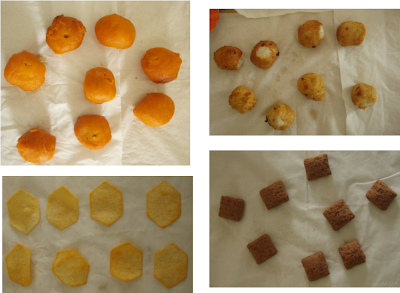 For the feature set, I chose something that can be extracted from all of the available images. These are pixel area, ratio of heigth and width, average red component (NCC), and average green component (NCC).
As can be seen in the pictures, the tissue does not have the same color for all the images. To correct this, I used the reference white algorithm to have a uniform tissue color in all the images. This can reduce the possible effect of lighting in both the training and test sets. After white balancing, the images are converted into grayscale and then binarized. To reduce the effect of poor thresholding, I used a closing operator with a 5x15 structuring element.
Feature Set
To calculate the pixel area, I just summed the binarized image. Also, to reduce the effect large variations in area, since pixel area is of magnitude 10^3 and the other features are only 10^0, I divided all area by the maximum area I obtained in the training set.
The ratio of height and width is computed as the maximum filled pixel coordinate vertically minus the minimum filled pixel coordinate vertically divided by its horizontal counterpart.
Since the cropped images I used don't have the same dimensions, I cannot just get the average red/green over the whole image. Instead, I considered only the average red/green of the ROI obtained from thresholding the binarized image.
The calculation of the feature vector is done similarly for the test images.
The feature vector of a class is represented by the mean of feature vector of all training images used.
The method used to classify the test images is just the Euclidean distance. The training feature set which have the shortest distance over the test features is the class of that test image.
For the feature set and the image processing method I used, I obtained 15 correct classifications out of 16 test images (a squidball was misclassified as piatos). Since I used a mean feature vector, large deviations from this mean can cause the program to classify an image to other classes.
For this activity, I give myself a grade of 10 since I was able to do it properly.
//Scilab code
getf("white_balance.sce");
parameters = []; //1 = area, 2 = h/w, 3 = r, 4 = g
for n = 1:4
for i = 1:4
I = imread("Images/" + names(n) + "/" + names(n) + string(i) + ".JPG");
I = ref_white(I); //white balancing
//Binarizing
I2 = I(:, :, 1) + I(:, :, 2) + I(:, :, 3);
I2 = I2/3;
I2(I2 > 0.75) = 2;
I2(I2 <= 0.75) = 1;
I2(I2 == 2) = 0;
//Closing operation
I2 = erode(dilate(I2, se), se);
//Area
area = sum(I2);
parameters(n, i, 1) = area;
//height/width
[v, h] = find(I2 == 1);
parameters(n, i, 2) = (max(v) - min(v))/(max(h) - min(h));
//average red and green (NCC)
ave = I(:, :, 1) + I(:, :, 2) + I(:, :, 3);
r = I(:, :, 1)./ave;
g = I(:, :, 2)./ave;
r = r.*I2;
g = g.*I2;
parameters(n, i, 3) = sum(r)/area;
parameters(n, i, 4) = sum(g)/area;
end
end
//just repeat everything for the test images
//use the following writes for the training set
fprintfMat("param1.txt", parameters(:, :, 1));
fprintfMat("param2.txt", parameters(:, :, 2));
fprintfMat("param3.txt", parameters(:, :, 3));
fprintfMat("param4.txt", parameters(:, :, 4));
//and the following for the test set
fprintfMat("param1-2.txt", parameters(:, :, 1));
fprintfMat("param2-2.txt", parameters(:, :, 2));
fprintfMat("param3-2.txt", parameters(:, :, 3));
fprintfMat("param4-2.txt", parameters(:, :, 4));
//The resutlts obtained above were saved in file param1.txt, ...
//Classifying the test images
parameters_train(:, :, 1) = fscanfMat("param1.txt");//area
parameters_train(:, :, 2) = fscanfMat("param2.txt");//h/w
parameters_train(:, :, 3) = fscanfMat("param3.txt");//mean(r)
parameters_train(:, :, 4) = fscanfMat("param4.txt");//mean(g)
for i = 1:4
for j = 1:4
m(i, j) = mean(parameters_train(i, :, j));
end
end
clear parameters_train;
normfactor = max(m(:, 1));
m(:, 1) = m(:, 1)/normfactor;
test(:, :, 1) = fscanfMat("param1-2.txt");
test(:, :, 2) = fscanfMat("param2-2.txt");
test(:, :, 3) = fscanfMat("param3-2.txt");
test(:, :, 4) = fscanfMat("param4-2.txt");
test(:, :, 1) = test(:, :, 1)/normfactor;
for i = 1:4
for j = 1:4
for k = 1:4
t(k) = test(i, j, k);
end
for l = 1:4
d = t' - m(l, :);
dist(i, j, l) = sqrt(d*d');//distance of image(i, j) on class l
end
end
end
correct = 0;
for i = 1:4
for j = 1:4
shortest = find(dist(:,j,i) == min(dist(:,j,i)));
if shortest == i
correct = correct + 1;
end
end
end
//code end
Wednesday, September 10, 2008
Basic Video Processing
For this activity, we need to capture on video some kinematic experiments which are easy to compute analytically and at the same time easy to image process. I used a video of an hollow cylinder rolling down an inclined plane.
The video is then cropped and then saved as jpg images using avidemux (freeware, http://fixounet.free.fr/avidemux/) (gif version shown above) Each image would then be processed in Scilab using one or more of the techniques in image processing learned from previous activities.
First I tried color segmentation but then the resulting binary image is not good to be processed. The color of the cylinder has almost the same color as the light reflection in the wood. (e.g. see the lower right portion of the image)
Next I tried grayscale thresholding. This one produced a more segmented ROI than the color segmentation so I used this method for the preliminary processing. After thresholding I applied an opening operator using a 5x15 structuring element. The resulting images are shown below.
 From the morphed images, I then calculated the center of the ROI and noted its pixel position. The horizontal-pixel location of the center of the ROI represents the displacement or distance traveled of the object. Each frame or image can be translated into time using the fps of the video camera.
The inclined plane has a length of about 480mm which is 240 pixels long in the image. So the distance to pixel conversion is 1px = 2mm. The camera has an fps of 24.5 so 1 frame (or 1 image) is equal to 1/24.5 sec.
I computed the acceleration of the object using the series of processed images using the formula change in velocity per change in time (dv/dt) where velocity is change in distance per change in time(dx/dt). The computed value of acceleration, using the pixel to mm and frame to sec conversion above, is 0.520m/sec. From physics books, we can see that the acceleration of a hollow cylinder rolling in an inclined plane is simple given by a = 0.5*g*sin(theta) where theta is the angle of inclination. In our setup, the angle is approximately 6 degrees so the acceleration is 0.512m/sec. The result from video processing gives an error of 1.6%.
For this activity, I give myself a grade of 10 since I was able to do it properly.
Tuesday, September 2, 2008
Color Image Segmentation
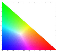
For this activity, we would do image segmentation using colors. To properly segment images by color, we need to transform the RGB colorspace into the normalized chromaticity space or NCC. Transformation is done by dividing each pixel channel with the sum of RGB (I) for that pixel(RGB -> rgb, where R/I = r and so on). The chromaticity can then be represented by only r and g as shown below.
 Two methods for image segmentation would be used, probability function estimation and histogram backprojection.
The image that would be segmented (test image):
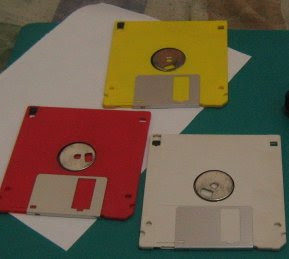 and the sample patch used, taken from the red diskette (region of interest, ROI) above:

A. Probability Function Estimation
In this method, we assumed a gaussian distribution for the r and g of the sample patch. Therefore, the probability that a pixel with chromaticity r belongs to the region of interest is:
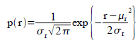 In the equation, the mean and standard deviation are computed from the sample patch and r is the r values of the test image. The equation above is also computed for the g channel. The probablity then that the pixel is in the region of interest is p(r)*p(g).
Using this equation and the test and sample image, I obtained the following image:
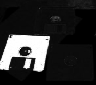 The portion from which the sample patch was obtained (red diskette) becomes white and the other color becomes black. Using this method worked very well for segmenting the region of interest from the image.
B. Histogram Backprojection
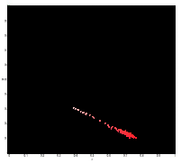
For this method, we first calculated the 2D histogram of the sample patch. For each pixel in the test image, we substitute the frequency value of the r and g from the 2D histogram of the patch.
The figure below shows the histogram of the sample patch superimposed on the NCC.
 After backprojection:
 The resulting image is not as accurate as the one obtained in probability function estimation but still it was able to separate the red diskette from the image.
//Scilab code
im = imread("sample--.jpg");
im2 = imread("image.jpg");
ave = im(:, :, 1) + im(:, :, 2) + im(:, :, 3);
r = im(:, :, 1)./ave;
g = im(:, :, 2)./ave;
b = im(:, :, 3)./ave;
ave = im2(:, :, 1) + im2(:, :, 2) + im2(:, :, 3);
ri = im2(:, :, 1)./ave;
gi = im2(:, :, 2)./ave;
bi = im2(:, :, 3)./ave;
mr = mean(r);
mg = mean(g);
stdr = stdev(r);
stdg = stdev(g);
pr = (1/(stdr*sqrt(2*%pi)))*exp(-((ri - mr).^2)./(2*stdr));
pg = (1/(stdg*sqrt(2*%pi)))*exp(-((gi - mg).^2)./(2*stdg));
prpg = pr.*pg;
scf(0);
imshow(prpg, []);
//Histogram Backprojection
//2D Histogram
r = r*255;
g = g*255;
imsize = size(r);
recurrence = zeros(256,256);
for i = 1:imsize(1)
for j = 1:imsize(2)
//x and y were re-oriented so that index (1, 1) would be at the origin of the
//normalize chromaticity plot
x = abs(255 - round(g(i, j)) + 1);
y = round(r(i, j)) + 1;
recurrence(x, y) = recurrence(x, y) + 1;
end
end
scf(1)
imshow(log(recurrence + 0.0000001), []);
//Histogram end
ri = ri*255;
gi = gi*255;
im3 = zeros(size(prpg));
imsize2 = size(ri);
for i = 1:imsize2(1)
for j = 1:imsize2(2)
x = abs(255 - round(gi(i, j)) + 1);
y = round(ri(i, j)) + 1;
im3(i, j) = recurrence(x, y);
end
end
scf(2);
imshow(im3);
//code end
I give myself a grade of 10 since I was able to do it properly ^_^
Collaborators: Raf Jaculbia
 Two methods for image segmentation would be used, probability function estimation and histogram backprojection.
The image that would be segmented (test image):
 and the sample patch used, taken from the red diskette (region of interest, ROI) above:
A. Probability Function Estimation
In this method, we assumed a gaussian distribution for the r and g of the sample patch. Therefore, the probability that a pixel with chromaticity r belongs to the region of interest is:
 In the equation, the mean and standard deviation are computed from the sample patch and r is the r values of the test image. The equation above is also computed for the g channel. The probablity then that the pixel is in the region of interest is p(r)*p(g).
Using this equation and the test and sample image, I obtained the following image:
 The portion from which the sample patch was obtained (red diskette) becomes white and the other color becomes black. Using this method worked very well for segmenting the region of interest from the image.
B. Histogram Backprojection
For this method, we first calculated the 2D histogram of the sample patch. For each pixel in the test image, we substitute the frequency value of the r and g from the 2D histogram of the patch.
The figure below shows the histogram of the sample patch superimposed on the NCC.
 After backprojection:
 The resulting image is not as accurate as the one obtained in probability function estimation but still it was able to separate the red diskette from the image.
//Scilab code
im = imread("sample--.jpg");
im2 = imread("image.jpg");
ave = im(:, :, 1) + im(:, :, 2) + im(:, :, 3);
r = im(:, :, 1)./ave;
g = im(:, :, 2)./ave;
b = im(:, :, 3)./ave;
ave = im2(:, :, 1) + im2(:, :, 2) + im2(:, :, 3);
ri = im2(:, :, 1)./ave;
gi = im2(:, :, 2)./ave;
bi = im2(:, :, 3)./ave;
mr = mean(r);
mg = mean(g);
stdr = stdev(r);
stdg = stdev(g);
pr = (1/(stdr*sqrt(2*%pi)))*exp(-((ri - mr).^2)./(2*stdr));
pg = (1/(stdg*sqrt(2*%pi)))*exp(-((gi - mg).^2)./(2*stdg));
prpg = pr.*pg;
scf(0);
imshow(prpg, []);
//Histogram Backprojection
//2D Histogram
r = r*255;
g = g*255;
imsize = size(r);
recurrence = zeros(256,256);
for i = 1:imsize(1)
for j = 1:imsize(2)
//x and y were re-oriented so that index (1, 1) would be at the origin of the
//normalize chromaticity plot
x = abs(255 - round(g(i, j)) + 1);
y = round(r(i, j)) + 1;
recurrence(x, y) = recurrence(x, y) + 1;
end
end
scf(1)
imshow(log(recurrence + 0.0000001), []);
//Histogram end
ri = ri*255;
gi = gi*255;
im3 = zeros(size(prpg));
imsize2 = size(ri);
for i = 1:imsize2(1)
for j = 1:imsize2(2)
x = abs(255 - round(gi(i, j)) + 1);
y = round(ri(i, j)) + 1;
im3(i, j) = recurrence(x, y);
end
end
scf(2);
imshow(im3);
//code end
I give myself a grade of 10 since I was able to do it properly ^_^
Collaborators: Raf Jaculbia
Thursday, August 28, 2008
Color Image Processing
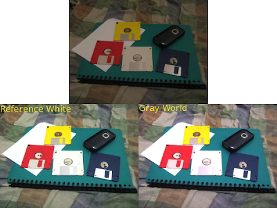
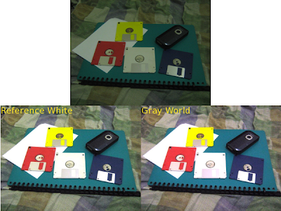
In this activity, we would be using 2 different algorithms for automatic white balancing. Reference white balancing is done by picking in the image the color that would represent white (reference white). The RGB values of this white would then be used as a divisor or balancing constants for the respective channels. Gray world algorithm is done by taking the average of each channel and then using these averages as the balancing constants.
These 2 algorithms were performed on images taken at different white balance of the camera. The white balance camera settings used were fluorescentH (which is redder compared to the bluer fluorescent setting), daylight, and tungsten.
FluorescentH
 Daylight
 Tungsten
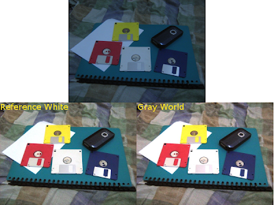 Both algorithms seems to perform relatively well, although the gray world algorithm needs some more tweaking in order to lower the brightness.
After trying both algorithms on colorful images, we then tried both on an image that contains few colors.
Blue Objects
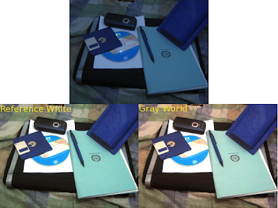 For low number of colors, the reference white algorithm seems to perform better. The gray world algorithm produced an image which is more reddish than the image produced by the reference white algorithm. I think reference white algorithm is better for images with few colors since it uses a fixed white color as the balancing factor unlike the gray world which averages all the colors present which would not produce a good result since it render colors biased to some colors.
//Scilab Code
I = imread(filename + ".JPG");
//Reference White
method = "rw-";
imshow(I);
pix = locate(1);
Rw = I(pix(1), pix(2), 1);
Gw = I(pix(1), pix(2), 2);
Bw = I(pix(1), pix(2), 3);
clf();
//Gray World
//method = "gw-";
//Rw = mean(I(:, :, 1));
//Gw = mean(I(:, :, 2));
//Bw = mean(I(:, :, 3));
I(:, :, 1) = I(:, :, 1)/Rw;
I(:, :, 2) = I(:, :, 2)/Gw;
I(:, :, 3) = I(:, :, 3)/Bw;
//I = I * 0.5; // for Gray world algorithm to reduce saturation
I(I > 1.0) = 1.0;
//code end
For this activity, I give myself a grade of 10 since all the objectives were accomplished. :)
Collaborators: Raf Jaculbia
Thursday, August 14, 2008
Stereometry
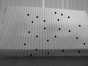
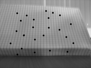
In this activity, we explore another method in 3d reconstruction, called stereometry. In this method, we try to reconstruct a 3d object using 2 images of it taken by the same camera at the same distance but with a different x position (assuming x is the parallel axis between the camera and the object). Using the same reference points (which I indicated by drawing dots on the graphing paper) from the 2 images, we can compute the z-axis or depth information.
The object I used was a graphing paper shaped like a box. The difference between the x axis position is 29mm.
 Since the focal length is automatically computed by the camera I used, I did not use the RQ factorization. The x values for the reference on both images and the calculated z values are tabulated below.
The object I used was a graphing paper shaped like a box. The difference between the x axis position is 29mm.

 Since the focal length is automatically computed by the camera I used, I did not use the RQ factorization. The x values for the reference on both images and the calculated z values are tabulated below.
| x1 | x2 | z |
| 128.519 | 47.0919 | −13.814 |
| 114.150 | 75.8309 | −29.354 |
| 132.625 | 72.4096 | −18.680 |
| 147.678 | 92.2532 | −20.294 |
| 141.52 | 76.5152 | −17.304 |
| 169.575 | 118.255 | −21.918 |
| 168.206 | 105.254 | −17.868 |
| 166.153 | 95.6745 | −15.960 |
| 203.104 | 149.047 | −20.808 |
| 203.788 | 145.626 | −19.339 |
| 218.157 | 153.152 | −17.304 |
| 220.210 | 153.152 | −16.774 |
| 253.055 | 191.471 | −18.265 |
| 253.055 | 203.104 | −22.518 |
| 266.056 | 214.052 | −21.629 |
| 271.530 | 214.736 | −19.805 |
| 287.268 | 220.210 | −16.774 |
| 282.478 | 233.895 | −23.153 |
| 316.691 | 262.634 | −20.808 |
| 312.586 | 264.003 | −23.153 |
| 350.904 | 292.058 | −19.114 |
| 360.484 | 296.163 | −17.488 |
| 383.749 | 322.849 | −18.470 |
| 363.221 | 311.901 | −21.918 |
Using linear interpolation, to fill in the gaps between reference points, and the cshep function(cubic scattered interpolation), I tried a 3d reconstruction of the object.
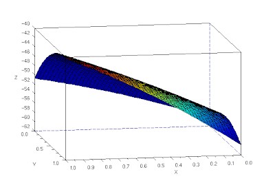 The 3d reconstruction is not that good (3d reconstructed image shown is not in the same angle as the original images). The corner is curved and the fold is not straight.
//Scilab code
b = 28.34;
f = 39.69;
d1 = fscanfMat("coords-image1.txt");
d2 = fscanfMat("coords-image2.txt");
x1 = d1(1, :);
x2 = d2(1, :);
y = d2(2, :);
z = b*f./((x2 - x1) + 0.00001);
x = x1;
np = 50;
xp = linspace(0,1,np); yp = xp;
[XP, YP] = ndgrid(xp,yp);
xyz = [x' y' z'];
XP = XP*40;
YP = YP*40;
ZP1 = eval_cshep2d(XP, YP, cshep2d(xyz));
xset("colormap", jetcolormap(64))
xbasc()
plot3d1(xp, yp, ZP1, flag=[2 2 4])
//code end
I give myself a grade of 7 since the blog was very late. :(
Thanks to Benj Palmares for the tip on using cshep instead of spline2d.
Thanks to Benj Palmares for the tip on using cshep instead of spline2d.
Subscribe to:
Posts (Atom)