Color Image Processing

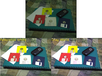
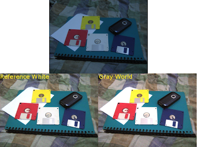
In this activity, we would be using 2 different algorithms for automatic white balancing. Reference white balancing is done by picking in the image the color that would represent white (reference white). The RGB values of this white would then be used as a divisor or balancing constants for the respective channels. Gray world algorithm is done by taking the average of each channel and then using these averages as the balancing constants.

These 2 algorithms were performed on images taken at different white balance of the camera. The white balance camera settings used were fluorescentH (which is redder compared to the bluer fluorescent setting), daylight, and tungsten.

FluorescentH
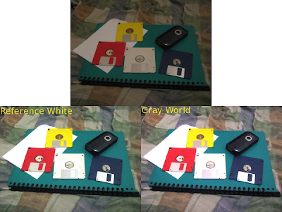
Daylight
Tungsten
Both algorithms seems to perform relatively well, although the gray world algorithm needs some more tweaking in order to lower the brightness.
After trying both algorithms on colorful images, we then tried both on an image that contains few colors.

Blue Objects
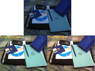
For low number of colors, the reference white algorithm seems to perform better. The gray world algorithm produced an image which is more reddish than the image produced by the reference white algorithm. I think reference white algorithm is better for images with few colors since it uses a fixed white color as the balancing factor unlike the gray world which averages all the colors present which would not produce a good result since it render colors biased to some colors.

//Scilab Code
I = imread(filename + ".JPG");

//Reference White
method = "rw-";
imshow(I);
pix = locate(1);
Rw = I(pix(1), pix(2), 1);
Gw = I(pix(1), pix(2), 2);
Bw = I(pix(1), pix(2), 3);
clf();

//Gray World
//method = "gw-";
//Rw = mean(I(:, :, 1));
//Gw = mean(I(:, :, 2));
//Bw = mean(I(:, :, 3));

I(:, :, 1) = I(:, :, 1)/Rw;
I(:, :, 2) = I(:, :, 2)/Gw;
I(:, :, 3) = I(:, :, 3)/Bw;
//I = I * 0.5; // for Gray world algorithm to reduce saturation
I(I > 1.0) = 1.0;
//code end

For this activity, I give myself a grade of 10 since all the objectives were accomplished. :)
Collaborators: Raf Jaculbia

Stereometry

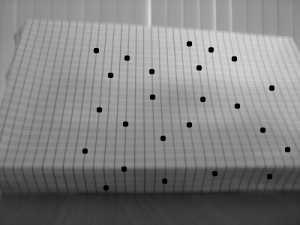
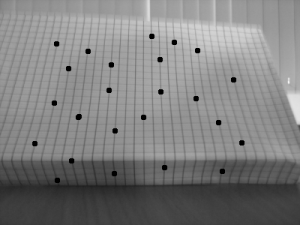
In this activity, we explore another method in 3d reconstruction, called stereometry. In this method, we try to reconstruct a 3d object using 2 images of it taken by the same camera at the same distance but with a different x position (assuming x is the parallel axis between the camera and the object). Using the same reference points (which I indicated by drawing dots on the graphing paper) from the 2 images, we can compute the z-axis or depth information.
The object I used was a graphing paper shaped like a box. The difference between the x axis position is 29mm.

Since the focal length is automatically computed by the camera I used, I did not use the RQ factorization. The x values for the reference on both images and the calculated z values are tabulated below.

x1	x2	z
128.519	47.0919	−13.814
114.150	75.8309	−29.354
132.625	72.4096	−18.680
147.678	92.2532	−20.294
141.52	76.5152	−17.304
169.575	118.255	−21.918
168.206	105.254	−17.868
166.153	95.6745	−15.960
203.104	149.047	−20.808
203.788	145.626	−19.339
218.157	153.152	−17.304
220.210	153.152	−16.774
253.055	191.471	−18.265
253.055	203.104	−22.518
266.056	214.052	−21.629
271.530	214.736	−19.805
287.268	220.210	−16.774
282.478	233.895	−23.153
316.691	262.634	−20.808
312.586	264.003	−23.153
350.904	292.058	−19.114
360.484	296.163	−17.488
383.749	322.849	−18.470
363.221	311.901	−21.918

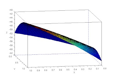
Using linear interpolation, to fill in the gaps between reference points, and the cshep function(cubic scattered interpolation), I tried a 3d reconstruction of the object.

The 3d reconstruction is not that good (3d reconstructed image shown is not in the same angle as the original images). The corner is curved and the fold is not straight.
//Scilab code
b = 28.34;
f = 39.69;
d1 = fscanfMat("coords-image1.txt");
d2 = fscanfMat("coords-image2.txt");
x1 = d1(1, :);
x2 = d2(1, :);
y = d2(2, :);
z = b*f./((x2 - x1) + 0.00001);
x = x1;
np = 50;
xp = linspace(0,1,np); yp = xp;
[XP, YP] = ndgrid(xp,yp);
xyz = [x' y' z'];
XP = XP*40;
YP = YP*40;
ZP1 = eval_cshep2d(XP, YP, cshep2d(xyz));
xset("colormap", jetcolormap(64))
xbasc()
plot3d1(xp, yp, ZP1, flag=[2 2 4])
//code end

I give myself a grade of 7 since the blog was very late. :(
Thanks to Benj Palmares for the tip on using cshep instead of spline2d.

Photometric Stereo

For this activity, we would reconstruct a 3D image using 2D images taken at different locations of point sources. The images used are shown below.
To get the elevation of the image, we used the following equation
where V is the matrix containing the locations of the sources, and I is the matrix containing the images. After this operation, we get a 3 row matrix corresponding to the xyz locations. To get a normal vector, we just need to divide each element in a column with the magnitude of that column. After this, a linear integral was used to obtain the z values. Plotting z with a 128x128 plane yields:
For this activity I give myself a grade of 10 since the reconstruction was quite accurate.
Collaborator: Raf Jaculbia
//Scilab code
chdir("C:\Documents and Settings\AP186user17\Desktop\ap18657activity13"); loadmatfile("Photos.mat");
V1 = {0.085832, 0.17365, 0.98106};
V2 = {0.085832, -0.17365, 0.98106};
V3 = {0.17365, 0, 0.98481};
V4 = {0.16318, -0.34202, 0.92542};
I(1, :) = I1(:)';
I(2, :) = I2(:)';
I(3, :) = I3(:)';
I(4, :) = I4(:)';
V = cat(1, V1, V2, V3, V4);
g = (inv(V'*V))*V'*I;
len = size(g);
len = len(2);
n = [];
mag = [];
for i = 1:len
mag(i) = sqrt(g(1, i)**2 + g(2, i)**2 + g(3, i)**2);
end
mag = mag';
n(1, :) = g(1, :)./(mag + 0.00000000000001);
n(2, :) = g(2, :)./(mag + 0.00000000000001);
n(3, :) = (g(3, :)./(mag + 0.00000000000001)) + 0.00000000000001;
dfdx = -(n(1, :))./n(3, :);
dfdy = -(n(2, :))./n(3, :);
dfdx = matrix(dfdx, [128, 128]);
dfdy = matrix(dfdy, [128, 128]);
lintfx = cumsum(dfdx, 2);
lintfy = cumsum(dfdy, 1);
z = lintfx + lintfy;
plot3d(1:128, 1:128, z)
//end of code