Color Image Segmentation

For this activity, we would do image segmentation using colors. To properly segment images by color, we need to transform the RGB colorspace into the normalized chromaticity space or NCC. Transformation is done by dividing each pixel channel with the sum of RGB (I) for that pixel(RGB -> rgb, where R/I = r and so on). The chromaticity can then be represented by only r and g as shown below.
Two methods for image segmentation would be used, probability function estimation and histogram backprojection.
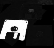
The image that would be segmented (test image):
and the sample patch used, taken from the red diskette (region of interest, ROI) above:

A. Probability Function Estimation
In this method, we assumed a gaussian distribution for the r and g of the sample patch. Therefore, the probability that a pixel with chromaticity r belongs to the region of interest is:
In the equation, the mean and standard deviation are computed from the sample patch and r is the r values of the test image. The equation above is also computed for the g channel. The probablity then that the pixel is in the region of interest is p(r)*p(g).
Using this equation and the test and sample image, I obtained the following image:
The portion from which the sample patch was obtained (red diskette) becomes white and the other color becomes black. Using this method worked very well for segmenting the region of interest from the image.

B. Histogram Backprojection
For this method, we first calculated the 2D histogram of the sample patch. For each pixel in the test image, we substitute the frequency value of the r and g from the 2D histogram of the patch.
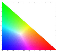
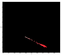
The figure below shows the histogram of the sample patch superimposed on the NCC.
After backprojection:
The resulting image is not as accurate as the one obtained in probability function estimation but still it was able to separate the red diskette from the image.

//Scilab code
im = imread("sample--.jpg");
im2 = imread("image.jpg");
ave = im(:, :, 1) + im(:, :, 2) + im(:, :, 3);
r = im(:, :, 1)./ave;
g = im(:, :, 2)./ave;
b = im(:, :, 3)./ave;
ave = im2(:, :, 1) + im2(:, :, 2) + im2(:, :, 3);
ri = im2(:, :, 1)./ave;
gi = im2(:, :, 2)./ave;
bi = im2(:, :, 3)./ave;

mr = mean(r);
mg = mean(g);
stdr = stdev(r);
stdg = stdev(g);

pr = (1/(stdr*sqrt(2*%pi)))*exp(-((ri - mr).^2)./(2*stdr));
pg = (1/(stdg*sqrt(2*%pi)))*exp(-((gi - mg).^2)./(2*stdg));
prpg = pr.*pg;
scf(0);
imshow(prpg, []);

//Histogram Backprojection
//2D Histogram
r = r*255;
g = g*255;
imsize = size(r);
recurrence = zeros(256,256);
for i = 1:imsize(1)
for j = 1:imsize(2)
//x and y were re-oriented so that index (1, 1) would be at the origin of the
//normalize chromaticity plot
x = abs(255 - round(g(i, j)) + 1);
y = round(r(i, j)) + 1;
recurrence(x, y) = recurrence(x, y) + 1;
end
end
scf(1)
imshow(log(recurrence + 0.0000001), []);
//Histogram end

ri = ri*255;
gi = gi*255;
im3 = zeros(size(prpg));
imsize2 = size(ri);
for i = 1:imsize2(1)
for j = 1:imsize2(2)
x = abs(255 - round(gi(i, j)) + 1);
y = round(ri(i, j)) + 1;
im3(i, j) = recurrence(x, y);
end
end
scf(2);
imshow(im3);
//code end

I give myself a grade of 10 since I was able to do it properly ^_^
Collaborators: Raf Jaculbia